Interpretable Deep Learning Part II: Visual Interpretability with Attribution Methods

In the previous post I identified different types of interpretability in deep learning. In this post, I focus on the advantages and shortcomings of one of the most popular types of post-hoc interpretability methods: feature attribution maps.

Feature attribution methods, or saliency methods, are one of the most popular local explanation methods for the interpretation of tasks of image classification or regression. These post-hoc techniques typically produce a heat-map showing how important each region or pixel of a particular picture is for its classification, i.e. which features of the input are most relevant for the resulting model output. In other words, they identify the regions of an image that a model is “looking at” in order to make its prediction.

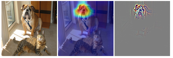
Figure 1. Input image and corresponding saliency maps obtained using two different feature attribution methods on a classification network. When considering the category “dog”, both visualization results show that the network focuses on the face of the dog. Figure source: Selvaraju et al. (2016). DOI: 10.1007/s11263-019-01228-7

Gradient-based methods

Gradient-based saliency methods are based on the calculation of the gradient (or its variants) of a particular neural network output, with respect to its input. Back-propagation is used to derive the contribution of the input features to a specific target neuron. For a classification task, the target of interest is usually the output neuron associated with the correct class, for a given sample. In the example of Fig. 1, the target used for the heatmaps is the output neuron associated with the class ‘dog’.

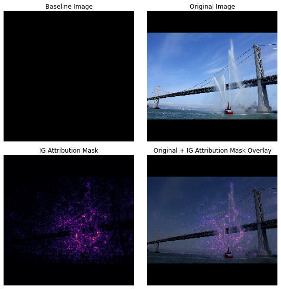
The simplest method of gradient-based attribution, simply referred to as Gradient·Input, is computed by taking the signed gradients of the output with respect to the input and multiplying them with the input itself. Integrated gradients [1] can be seen as an extension of this method, and are defined as the integral of the gradients from a given baseline to the input image. This baseline is defined by the user and is often chosen to be zero (an all black image). A series of images are linearly interpolated between the baseline and the original image, and the resulting Gradients are summed across this series of interpolated images, as exemplified in Fig. 2.

Figure 2. Feature attribution using the Integrated Gradients method on an image of a fireboat. The baseline chosen to calculate the interpolated images is a black image. The resulting saliency map, also shown superimposed over the input image, highlights the pixels comprising the boat’s water cannons and jets of water as being the most important to its decision to classify the image in the fireboat category. Figure source

DeconvNets are a saliency method similar to the “Gradients” approach, except for a difference in backpropagation through the ReLU nonlinearity, where backpropagation is only performed for positive gradients (negative gradients are zeroed out). Guided Backpropagation [2] is a method where backpropagation is guided by both the input and gradients, by applying the ReLU operation to the gradients itself during the backward pass (like in DeconvNets) and also handling ReLUs by restricting to only positive elements in the preceding feature maps (like in “vanilla” Gradients).

Grad-CAM [3] is a gradient-based saliency method that computes the gradients of the target output with respect to the final convolutional layer of a network. The layer activations are weighted by the average gradient for each output channel and the results are summed over all channels to produce a coarse heatmap of importance for prediction of a class. The result of a Grad-CAM operation is therefore a heatmap of the same dimensions (except in number of channels) as those of the final convolutional layer of the network, but is frequently upsampled to correspond to the original input size, in order to allow for a better visualization.

Pertubation-based methods

Perturbation-based methods are generally model-agnostic methods, that directly compute the attribution of an input by removing, masking or altering it, and then running a forward pass on the new input, comparing the difference in output to the original instance.

The most popular perturbation-based method is occlusion. Occlusion is a perturbation-based method that involves replacing portions of an image with an occlusion block of a given baseline value, and obtaining the output when the occluded image is passed through the network. A heatmap is formed using the difference between the output attributed to the original image and the output computed for the occluded image, for different positions of the occlusion block across the input image. The most simple case consists of using a black square of small dimensions that “slides” across the image, occluding different regions of the image at each iteration. Instead of a simple black square, occlusion can also be performed by blurring portions of the image, substituting values by other values present in the image, or by swapping different features in an image.

Occlusion perturbation has the strong advantage of being a simple attribution method that can be used to visualize the decisions of any network, as it does not require any information about the insides of the network. The main disadvantage of this method is that it is more computationally intensive than some gradient-based methods, because multiple instances of the input need to be created and passed through the network.

Shortcomings of attribution methods

Attribution methods are very popular methods of visual explanation, and indeed can identify relevant information about the decisions of models. Moreover, they provide a type of quantification (i.e. importance for each pixel), and are capable of providing explanations that are helpful to both end users and model developers. However, there are some limitations inherent to this type of method.

First of all, since a saliency map is usually conditioned on only one input (i.e. one image), humans have to manually assess each resulting heatmap in order to draw a class-wide conclusion, or look at averaged results when it makes sense to do so (for example, if one is dealing with registered images i.e. images that overlap spatially).

Furthermore, recent work [4] has demonstrated that simple data processing steps that should be theoretically meaningless, such as simple shifts in mean intensity in MNIST images, can cause saliency methods to compute significantly different visual explanations.

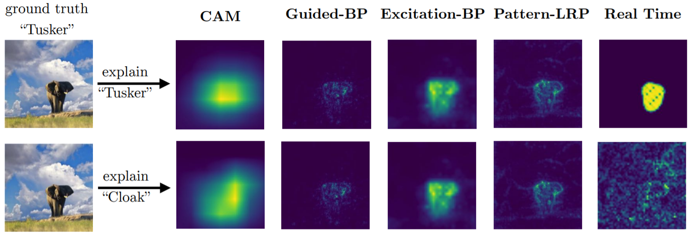
Another known flaw of these methods is mode collapse: these types of gradient-based approaches can often generate high-response outputs even if a non-existing class is requested for explanations, as exemplified in the image below, from a study by [5]:

Figure 3. Comparison of several saliency methods on an image of a wild Tusker. When explaining the ground-truth class ”Tusker”, the methods can localize the object correctly (first row). But when asked to explain a non-existing class (in this case “Cloak”), these approaches can still generate a similar saliency map, or generate dispersive and irregular artifacts. Figure source: [5]

In this example it is clear that no cloaks are visible in the image of a Tusker elephant in the wild. However, computing an attribution map using a target of interest that is not present in the image results in heatmaps that are similar to the ones computed for the true class, for popular saliency methods such as CAM and Guided Back Propagation.

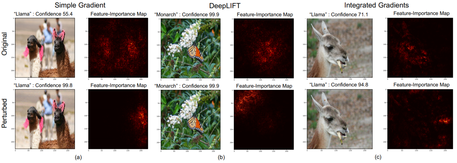
Saliency maps may also be vulnerable to adversarial attacks, as investigated by Ghobarni et al. [6]. In this study, the authors engineer perturbation noise that does not result in a change of label on the input images, but that can result in saliency maps that shift dramatically to highlight features that would not be considered salient by human perception. In other words, inputs are assigned the same predicted label, yet with very different interpretations. The adversarial attacks are applied to popular gradient-based feature attribution methods, as shown in Fig. 4.

Figure 4. Example of adversarial attacks against feature-attribution maps developed by Ghorbani et al. The top row shows the original images and their saliency maps using 3 different methods, considering their true labels (‘Llama’, ‘Monarch’, and ‘Llama’ again). The bottom row shows the perturbed images, with perturbations specifically designed to not change the predicted label. The corresponding saliency maps change completely when the noise is added, showing the fragility of these methods to adversarial attacks. Source: [6]

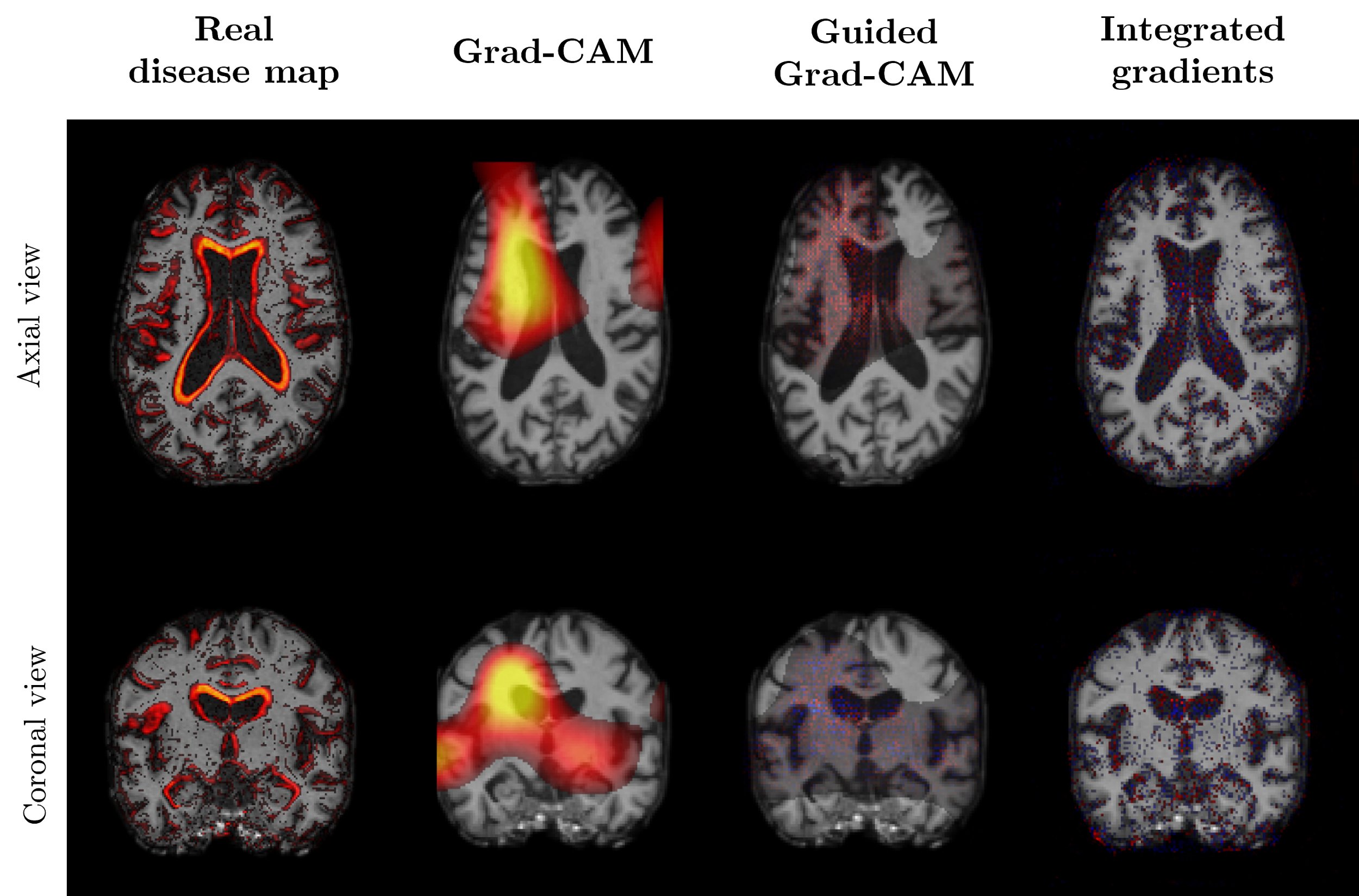
Finally, saliency methods may be the state-of-the-art visual attribution method for single class classification tasks and when the inputs contain a single instance of that class, but their performance worsens when dealing with multi-class prediction, or when multiple instances of a class are present in a single data input (Fig. 5.).

Figure 5. When applied to images classified as Alzheimer’s Disease (characterized by changes in multiple regions of the brain, as well as high inter-subject variability), post-hoc saliency methods fail to capture all class-relevant features, and produce noisy heatmaps.

This sort of problem can be encountered in classification of diseases that are manifested with various symptoms or in different regions - take for example complex brain diseases: an issue here is that the same features aren’t present in all datasets, so saliency methods will not pick up on the less common ones, even if they are important to explain a diagnosis (Fig 5). This is not the case with images of single tumors or focused lesions, where these sort of methods can prove more efficient.

Finally, these saliency methods do not take into account any causal interactions between different features occurring in the same input and between them and the corresponding output.

References

1. Sundararajan M. et al. (2017). Axiomatic Attribution for Deep Networks. ICML.
2. Zeiler, M. D., & Fergus, R. (2014). Visualizing and understanding convolutional networks. Computer Vision - ECCV. DOI: 10.1007/978-3-319-10590-1_53
3. Selvaraju, R. et al. (2019). Grad-CAM: Visual Explanations from Deep Networks via Gradient-Based Localization. International Journal of Computer Vision. DOI: 10.1007/s11263-019-01228-7
4. Adebayo, J. et al. (2018). Sanity checks for saliency maps. NIPS 2018 Proceedings
5. Wang, Y. et al. (2018). Learning attributions grounded in existing facts for robust visual explanation. Workshop on Explainable Artificial Intelligence - XAI 2018
6. Ghorbani, A. et al. (2019). Interpretation of neural networks is fragile. Proceedings of the AAAI Conference on Artificial Intelligence. DOI: 10.1609/aaai.v33i01.33013681